Expected Value Finish

Welcome back to the third and last in a series of posts from our good friend Craig Hilsenrath at Option Workbench. In the first two Craig introduced us to the concept of Expected Value and why it is important to options trading and helped us understand the math behind the scenes. In this final post he gives us the rest of the equation so to speak. We here at Tradier believe the more you know the better off you are. Look for more exciting educational posts to come.

Expected Value and Option Strategies
Recalling the definition of expected value, the weighted average value of a variable, we
first need to determine which variable we want to model. Since the goal of placing a
trade is to earn a profit we want to determine what the expected profit of the trade is before putting it on. If the expected profit is positive then, on average, we can expect to
make a profit on this trade. If the expected profit is negative then we should NOT do the
trade.

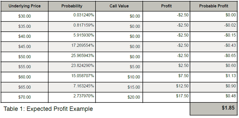
As a simple example consider an at-the-money long $50 strike call position with ninety
days to expiration put on for a $2.50 debit. Since the value of an option is partially
derived from the price of the underlying, the expected profit can be calculated by using
the underlying price as the random variable. The role of volatility, another important
input into the calculation of the value of an option, will be discussed later. Table 1 shows
how the expected profit at expiration can be calculated. The table shows nine possible
values of the underlying stock at expiration, the probability that the stock will be at that
price in ninety days, the value of the call at expiration at the underlying price and the
profit/loss of the position. The final column shows the product of the profit and
probability columns. At the bottom of the Probable Profit column is the weighted
average sum for an expected profit of $1.85.

Analysis of the data in Table 1 reveals some important properties of the expected profit
calculation. Two principal differences between the gaming examples above are evident.
First, in practical terms, “all the possible values” of the variable cannot be known. Since
the price of the stock can take on any value between zero and infinity, a range of prices
will need to be selected that will give the trader enough confidence in the resulting
expected profit. In statistics this range is called a confidence interval. ! !
In any trading endeavor a prediction about the future value of some variable must be
made. An option trader is typically attempting to make a profit over a range of the
underlying price. Predicting this range depends on an expectation of the volatility of the
underlying price over time. Since volatility measures the standard deviation of price
returns, standard deviations can be used to determine the range of prices for the desired confidence interval. Professional risk managers typically use an interval from
-3.0 to +3.0 standard deviations because that range corresponds to a 99.7%
confidence. From a statistical perspective this means that the underlying price should
fall within that range for 99.7% of the observations. Equation 1 shows how to calculate
what the underlying price is for a given number of standard deviations.
Equation 1


where:

    P0 = The current price of the underlying.
    e = The natural exponential constant.
    σ = The volatility for the period.
    n = The number of standard deviations.

Assuming an annualized volatility of 25% --14.94% for the 90-day period using the square
root of time rule, σT = σ√(90/252) -- and a currentprice of $50 the price ranges from $31.94 to
$78.28 for the 99.7% confidence interval. The next question that arises is how to pick the
prices in between the end points. UsingEquation 1 Pn can be determined for any number of standard deviations. So the objective is to pick some increment of n that will result in enough prices to obtain an acceptable sampling but not so many as to make the calculation too time consuming. As it turns out this is closely related to how the probability of the underlying price moving to that level is determined.

Determining the probabilities is the second difference between the gaming examples
and the expected profit calculation. Whereas the probabilities for the casino games are
known and constant, the probabilities used to calculate expected profit are dependent
upon an assumption about the price volatility of the underlying asset.

Determining the Probabilities
In 1973 Fisher Black and Myron Scholes published a paper defining the now famous
Black-Scholes option pricing model. One of the characteristics of the Black-Scholes
model is that it assumes that the underlying asset’s daily returns follow a log-normal
distribution. The reason for this assumption is so that the model can estimate the
probability that the option will expire in the money and earn a profit for the option buyer.
There are two concepts that need to be understood in order to comprehend how the
probabilities are calculated. The first, the probability density function or PDF, is defined
as a function that describes the relative likelihood for a random variable to take on a
given value. The figure below shows a typical normal probability density function. The xaxis
shows the change of the variable, the underlying price return in our case, in
standard deviations. The Greek letter μ is used to represent the mean or average
change.

In the context of the Black-Scholes pricing model this means that the distribution of the
natural logarithm of daily returns conforms roughly to the normal distribution. What the
PDF tells us is the frequency at which we can expect the log return to change by a
certain number of standard deviations. However, this is not the probability. As indicated
in the diagram, the probability is represented by the area under the PDF. Taking the sum
of the numbers representing the area between -3 and +3 standard deviations results in
the 99.7% confidence interval.

To calculate the probabilities we need to know the area under the PDF curve for the
number of standard deviations represented by the price change. This is accomplished
by using the Cumulative Density Function or CDF. Figure 2 below shows the CDF for
the normal distribution depicted in Figure 1.

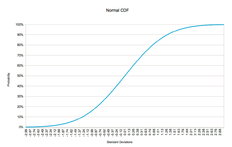
It is important to note that a point on the CDF designates the probability of the variable
being less than or equal to the corresponding number of standard deviations. Therefore,
the probability of the price moving zero or less standard deviations is 50%. Likewise, the
probability of the price moving more than zero standard deviations is 50%.
How does this help us to derive the probabilities we need to calculate the expected
profit? Another property of the CDF is that it can be used to calculate the probability of
the variable falling between two points on the curve. This is accomplished by
subtracting the probability at the lower end of the interval from the probability at the
upper end of the interval. In mathematical terms:

Equation 2
F(xL < x ≤ xU) = F(xU) - F(xL)

Referring back to Table 1, the probabilities stated in the second column were actually
determined by using the formula above and a $5 interval. So the 23.82% probability of
the underlying being at $55 is actually the probability of the underlying being between
$50 and $55. For that simple example a $5 interval was sufficient. However for actual
trading a much smaller interval is needed.

Before deciding on what interval is appropriate there is a tradeoff that needs to be
considered. In the example in Table 1 nine values for the underlying price were
evaluated. In each step the probability, the value of the call, the theoretical profit and the probable profit were calculated. The probable profit for each row is the probability times
the profit from the weighted average sum formula above. Computing the probability and
the value of the call are both complex, multi-step calculations. As such, performing
these calculations too many times can consume a great deal of computational resources.

Since a stock price cannot move less than one penny it may be tempting to pick a small
interval around a penny. For example, the interval p - 0.005 < p ≤ p + 0.005 will yield a
very precise probability. In the previous example the range from $31.94 to $78.28 will
result in 4,634 prices to consider. If the volatility assumption is increased from 25% to
50% annualized the number of prices increases to 10,214. So changing the volatility
assumption can make a big difference in the number of calculations that are performed.
When contemplating the wide dispersion of possible underlying prices and the variety of
volatility scenarios, it is easy to see that using the price-based interval can lead to vastly
different consumption of computational resources.

As it turns out the differences in the probabilities using the $0.01 range are so
minuscule that the extra computations are not worth the effort. A better solution that
results in more than adequate results is to divide the range into equal size chunks. The
objective is to choose a chunk size that results in a small enough difference in the
probabilities without incurring undue computational expense.

Given that the endpoints of the price range are defined in terms of standard deviations,
it makes sense to use an increment of standard deviations to divide the range. For
example, using 1/128 of a standard deviation (a nice round computer number), divides
the six standard deviation range into 768 chunks. Table 2 below shows a revision to the
long call example above. A new column showing the number of standard deviations has
been added. As the table shows this long call still has a positive expectation. If a trader
could buy a call like this many times, on average, a profit of $76.34 per contract would
be expected.

Fat Tail Distributions
The preceding examples assume that the price returns of the underlying asset follow a
log normal distribution. Very few, if any, equities or instruments of any asset class
actually exhibit this behavior. In the real world price fluctuations are subject to shocks
caused by corporate actions, natural disasters, political turmoil and other exogenous
events. Single day price moves of four or more standard deviations are not uncommon.
This means that the probability of extreme changes is higher than would be predicted by
the normal distribution, leading to the understatement of the probable profit at the
extremes or tails of the distribution.

This fact calls into question the value of using the standard statistical techniques
outlined above. In fact, there are many techniques employed by professional risk
managers that apply adjustments to the normal distribution. These so-called parametric
approaches attempt to account for extreme return fluctuations in a generalized way.

There is also a non-parametric or empirical approach that can be used. This method
uses historical data to construct the probability density and cumulative density curve.
The empirical approach is not generally used by professional risk managers because
they are typically dealing with large portfolios of diversified assets and a more
generalized approach is needed. However, for the purposes of calculating the expected
profit for an option strategy, using empirical data is a reasonable technique.

The Empirical Probability Density
In the normal PDF exhibited above the tails of the distribution decline smoothly and
approach zero as the number of standard deviations approach negative and positive
infinity. In a fat tail probability density the extremes of the distribution are elevated to
take into account periodic extreme moves in asset returns. The chart below is an
example of an empirical, fat tail probability density for the S&P-500 index. The daily
return data were collected for 10-year period ending in June of 2013. In the histogram
the eight standard deviation range from -4.0 to +4.0 is divided into 128 buckets. The
height of the bars indicates what percentage of the return data falls into each bucket.
The histogram is superimposed over a normal distribution to illustrate the differences in
the tails. From Equation 1, the number of standard deviations is calculated using
Equation 3.

Equation 3



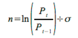
where:
Pt = The closing price for the current day
Pt-1 = The closing price for the previous day
σ = The standard deviation of the returns.


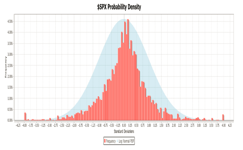
Each day’s closing price is compared to the previous day’s price to determine the return
in terms of standard deviations. Each bucket encompasses a 0.0625 standard deviation
range, the eight standard deviation total range divided by 128 buckets. To determine in
which bucket a reading belongs, subtract the minimum value from the reading and
divide by the bucket range. Changes greater than or equal to 4 standard deviations are
counted in the highest bin. Changes of more than -4 standard deviations are placed in
the lowest bin.

The Empirical Cumulative Density Curve
Using the empirical probability density a cumulative density curve can be constructed.
The following chart shows the cumulative density curve derived from the probability
density above. The red line depicts the empirical cumulative density curve and the blue
line shows the log normal CDF for comparison. One difference between the two that is
immediately apparent is that the log normal CDF is smooth and continuous whereas the
empirical curve neither smooth nor continuous. The $SPX probability density used to
construct the cumulative density curve is missing some bars in some of the upper end
buckets. Even if all the buckets contained data the empirical cumulative density curve
would still not be continuous. Recall that to calculate the expected profit a very small
increment of standard deviations was used. Since the log normal CDF is a continuous
function a value for any number of standard deviations can be computed. This is not the
case for the empirical cumulative density curve. For values that are not points on the
empirical cumulative density curve curve an interpolation method will need to be used to
determine the probabilities.

One of the tradeoffs between using an empirical cumulative density curve versus the log
normal CDF is that the former offers an accurate approximation of “tail risk” while the
latter offers a better approximation of the probabilities. Another point to consider is what
data are used to construct the empirical probability density. If the $SPX probability
density were constructed using only 3 years of daily data the 2008 financial crisis would
not have been included. There are valid reasons for selecting both time frames
depending circumstances. One could also choose to use weekly or monthly returns to
construct the probability density. All of these choices will affect the shape of the
empirical cumulative density curve.

In summary, a fat tail distribution can offer a better estimate of expected profit but there
is not one, correct fat tail distribution. An option trader who would like to use a fat tail
distribution to calculate expected profit should be aware of what assumptions were
made in constructing the empirical probability density.

Expected Return
While having a positive expected profit is preferable it is not always sufficient. A trade
with a positive expectation can still result in a loss so attention must be paid to risk.
Expected return, the expected profit divided by the risk, tells an option strategist
whether the expected profit is worth the risk.
In the long call example above the risk is $2.50, the cost of the call. So the expected
return is approximately 30.54%. Suppose now that the cost of the call was actually
$3.75. That would reduce the expected profit to approximately $0.14 for an expected
return of 3.63%. Even though the trade still has a positive expectation, a return of 3.63%
does not seem worth the risk. This conclusion is subjective and has to be weighed
against alternative uses of the trading capital. Perhaps 3.63% is not a bad return given
general market conditions. This type of comparison highlights another use of expected
return.

The expected return of positions with different strikes, expiration dates and even
different underlying assets can be compared using expected return. The final step is to
normalize the return. Suppose a trader wants to compare the long call analyzed above
with a 60 day call for a price of $1.85. The expected profit of the new call position is
approximately $0.39 for an expected return of 21.26%. The question is would the trader
prefer a return of 21.26% over 60 days or 30.54% over 90 days. The reason this needs
to be considered is that the proceeds from the 60 day trade can be reinvested for the
thirty days between the two expiration dates. Equation 4 shows how to calculate the
compound annualized return.
Equation 4


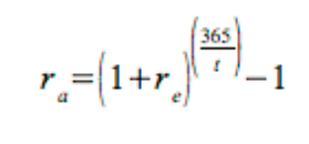
where:
re = The expected return.
t = The number of days over which the expected return is realized.
Using equation 4, the original 90 day trade yields 194.69% on an annualized basis and
the 60 day trade yields 223.01%. This shows that the 60 day call has an edge over the
90 day call and the trader should prefer the new position.

Conclusion
Using expected value can help people to predict possible outcomes in many different
areas. Casinos use probability and the expected value of the games that gamblers play
to give the house an edge. In the same way option strategists can use expected return
to establish an edge in their portfolios. By carefully establishing and maintaining
positions with positive expected returns, option traders can use probability and statistics
to enhance portfolio returns, and in a sense, be the house.

 Many thanks and stay tuned for more from other guest contributors.

Craig Russell